Level: Intermediate Stack: Apache Spark 3.4+, Scala 2.12
TL;DR: Adaptive Query Execution re-optimizes your Spark jobs at runtime, after each shuffle. Three features, zero code changes, massive impact.
Spark AQE: The 3 Features That Make Static Query Plans Obsolete
Why Static Plans Fail at Scale
Spark’s query optimizer — Catalyst — produces an execution plan before your job runs. It relies on statistics collected at planning time: estimated row counts, estimated data sizes, column cardinality. These estimates drive critical decisions: how many partitions to create, which join algorithm to use, whether a partition is skewed.
The problem is fundamental. At planning time, Catalyst doesn’t know:
- How many rows survive your filters
- What the actual output size of a shuffle will be
- Whether your join key has a skewed distribution at runtime
The result: jobs optimized for a world that doesn’t exist. Too many partitions for small data, the wrong join algorithm for filtered tables, no defense against data skew.
AQE — Adaptive Query Execution — was designed to fix this. Introduced in Spark 3.0 and enabled by default from Spark 3.2, it turns query optimization from a one-shot pre-execution step into a continuous feedback loop at runtime.
This post covers all three AQE features, their configuration, and exactly what to look for in the Spark UI to verify each one is working.
The AQE Mechanism: QueryStages and Shuffle Boundaries
Before diving into features, the key mental model: AQE operates at shuffle boundaries.
Spark divides your query plan into QueryStages — segments of the plan separated by shuffle operations. Each shuffle write is a natural pause point where real data statistics become available (actual bytes per partition, actual record counts, actual key distribution). AQE reads these statistics at each boundary and re-optimizes the downstream plan before the next stage executes.
┌──────────────────────────────────┐
│  Stage 1: Scan + Filter + Map    │
└─────────────────┬────────────────┘
                  │ shuffle write
          ┌───────▼───────────┐
          │  AQE checkpoint   │  ← real stats: bytes/partition, row count, key distribution
          └───────┬───────────┘
                  │ re-optimized plan
┌─────────────────▼────────────────┐
│  Stage 2: Join / GroupBy         │  ← runs with corrected plan
└─────────────────┬────────────────┘
                  │ shuffle write
          ┌───────▼───────────┐
          │  AQE checkpoint   │  ← another re-evaluation
          └───────┬───────────┘
┌─────────────────▼────────────────┐
│  Stage 3: Final Aggregation      │
└──────────────────────────────────┘
A plan with 3 shuffles gets 3 independent optimization passes. The more complex your pipeline, the more AQE has to work with.
One important boundary case: persist() materializes data in memory or on disk but does not create a shuffle boundary. AQE cannot see statistics across a cache and will not re-optimize at that point.
Feature 1 — Dynamic Partition Coalescing
The Problem: The 200-Partition Tax
spark.sql.shuffle.partitions defaults to 200. Spark creates exactly that many partitions after every shuffle — for 500 MB of data, for 500 KB of data, for anything in between.
For small-to-medium datasets, this means hundreds of tasks doing milliseconds of work. The cost of launching and scheduling those tasks often exceeds the cost of doing the work itself.
shuffle.partitions = 200
Data after shuffle = 400 MB

→ 200 partitions × ~2 MB each
→ 200 task launches, JVM overhead, scheduler pressure
→ Wasted parallelism on trivially small partitions
Before AQE, the only fix was manually tuning shuffle.partitions per job — and re-tuning every time data volume changed.
What AQE Does
After each shuffle write, AQE reads the actual partition sizes from the shuffle map output files. It then applies a greedy merge algorithm: scan partitions left-to-right, accumulate until the target size is reached, close the group, start a new one.
Before coalescing (shuffle.partitions = 200):
[2MB][1MB][3MB][2MB][1MB][2MB][3MB]... × 200 partitions

advisoryPartitionSizeInBytes = 128 MB

After coalescing:
[~100MB merged][~98MB merged][~104MB merged][~98MB merged]
→ 4 partitions instead of 200
→ Next stage launches 4 tasks, not 200
The merge happens between stages, transparently. Your code is unchanged.
Spark UI — Without AQE
Here’s what the physical plan looks like with AQE disabled. The Exchange node shows 200 partitions, and the downstream WholeStageCodegen takes 3.6 seconds — extreme variance driven by scheduling overhead across 200 tasks, not actual computation:
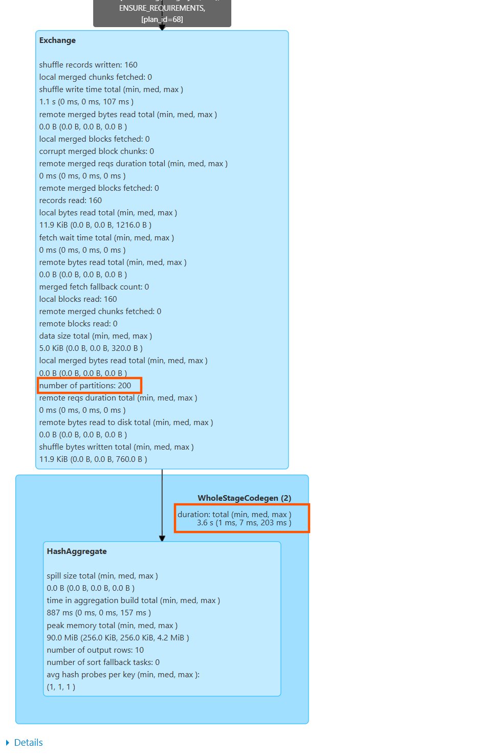
The Exchange writes 200 shuffle partition files for 5 KiB of real data. Each task does ~25 bytes of work.
Spark UI — With AQE
With AQE enabled, the AQEShuffleRead node appears between the Exchange and the next operator. It shows the coalescing result directly:
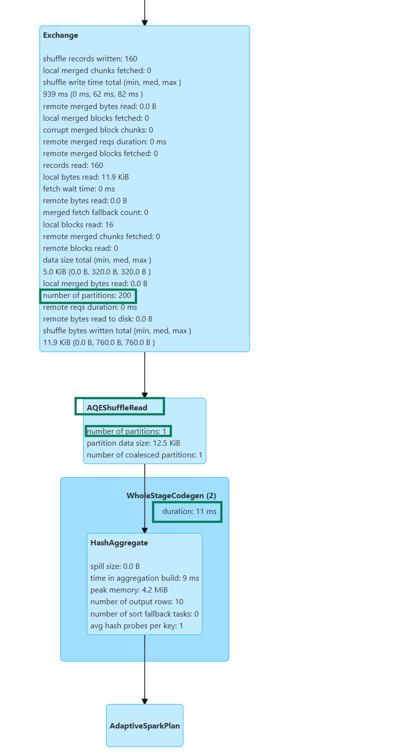
Key metrics to note:
number of partitions: 1— AQE merged all 200 into a single partitionnumber of coalesced partitions: 1— confirms the coalescing eventpartition data size: 12.5 KiB— the actual data size AQE measured before merging- WholeStageCodegen duration: 11ms — down from 3.6s
Spark UI — Stages Comparison
The Stages tab makes the before/after contrast impossible to miss:

- Stage 4 (AQE OFF): 200 tasks, 1s total duration
- Stage 7 (AQE ON): 1 task, 31ms total duration
Same query. Same data. 199 fewer task launches.
Configuration
// Core setup
spark.conf.set("spark.sql.adaptive.enabled", "true")

// Set HIGH — AQE will reduce this at runtime
// Rule of thumb: target ~128 MB per partition BEFORE coalescing
// 100 GB shuffle → shuffle.partitions = 800
spark.conf.set("spark.sql.shuffle.partitions", "600")

// Target size per merged partition (default: 64 MB → use 128 MB in prod)
spark.conf.set("spark.sql.adaptive.advisoryPartitionSizeInBytes", "134217728")

// Floor: never create a partition smaller than this
spark.conf.set("spark.sql.adaptive.coalescePartitions.minPartitionSize", "1048576")
The mental model:
| Parameter | Role |
|---|---|
shuffle.partitions |
The ceiling you set — high enough to avoid OOM before coalescing |
advisoryPartitionSizeInBytes |
The target AQE aims for — what you want each output partition to be |
| Result | AQE reduces shuffle.partitions → actual partitions needed |
Key Constraints
- Only applies to the DataFrame/Dataset API — RDD operations (
groupByKey,flatMap) are invisible to Catalyst persist()does not create a shuffle boundary — AQE cannot optimize across it- AQE coalesces after the shuffle write. If partitions are already too large during the shuffle (causing spill/OOM), you need a higher
shuffle.partitionsvalue before relying on coalescing
Feature 2 — Dynamic Join Strategy Switching
The Problem: Catalyst Estimates the Wrong Table Size
Spark chooses between join algorithms at planning time based on estimated table sizes:
- Sort-Merge Join (SMJ): Default for large-large joins. Requires two network shuffles. Cost: O(N log N) sort + network I/O on both sides.
- Broadcast Hash Join (BHJ): Used when one table fits in executor memory. The small table is broadcast to all executors; each executor performs a local hash lookup. Cost: O(N) hash lookup, zero network shuffles.
BHJ is 3–5x faster than SMJ when applicable. The problem: Catalyst estimates table size before your filters execute.
Table B estimated size at plan time: 500 MB → Catalyst picks SMJ
Table B actual size after filters:     5 MB → BHJ would have been 4x faster

Without AQE: SMJ runs anyway. You pay 2 network shuffles for 5 MB of data.
What AQE Does
After Stage 1 executes (scan + filter), AQE reads the actual shuffle output size of the filtered table. If it’s below autoBroadcastJoinThreshold, AQE switches the join strategy at runtime — converting the planned SMJ into a BHJ, even if Catalyst originally chose otherwise.
Plan time:    SMJ(A, B)           ← Catalyst's estimate: B is large
Runtime:      filter(B) → 50 KB  ← AQE reads real shuffle output
AQE rewrite:  BHJ(A, broadcast(B)) ← dynamic strategy switch
No code change. No query rewrite. AQE replaces the physical operator mid-execution.
Spark UI — Without AQE (SortMergeJoin)
With AQE disabled, Catalyst commits to SMJ at planning time. Both tables go through a full shuffle:
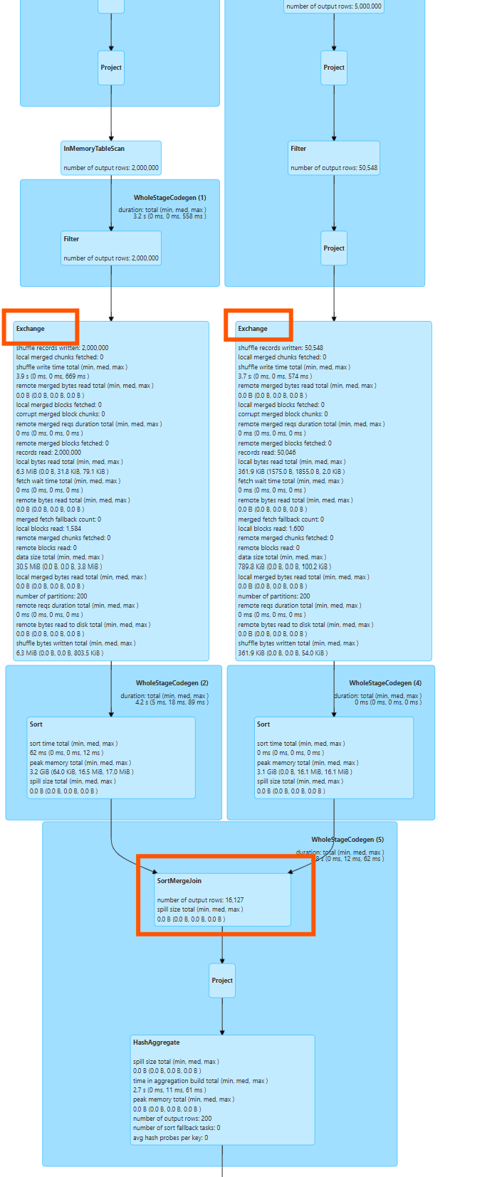
The two red-boxed Exchange nodes are the tell: both tables shuffled over the network before the join can happen. SortMergeJoin sits at the bottom consuming both sorted streams. number of partitions: 200 on each exchange.
Spark UI — With AQE (BroadcastHashJoin)
With AQE enabled, the physical plan is rewritten at runtime:
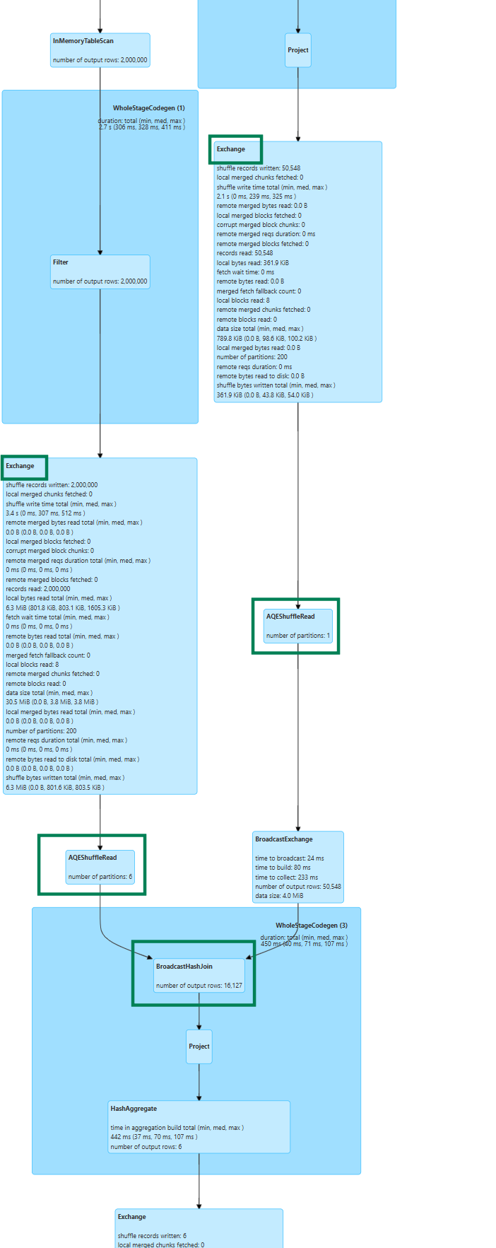
The green-boxed nodes tell the story:
- Left side:
AQEShuffleRead: 6 partitions— coalescing also fired on the large table - Right side:
AQEShuffleRead: 1 partition→BroadcastExchange— AQE measured 50,548 rows / 4.0 MiB at runtime and switched strategy BroadcastHashJoinreplaces SortMergeJoin — zero shuffle on the small table side
Note: AQE applied two optimizations simultaneously — it switched SMJ → BHJ and coalesced the large table from 200 → 6 partitions. Both happen at the same shuffle boundary checkpoint. The features compose.
Configuration
// Broadcast threshold: if the smaller side is below this after filters, AQE switches to BHJ
// Default: 10 MB — too conservative for most production workloads
// Recommended: 50 MB
spark.conf.set("spark.sql.autoBroadcastJoinThreshold", "52428800") // 50 MB
SMJ vs. BHJ Decision Table
| Condition | Join Strategy |
|---|---|
| Both tables large (post-filter) | SMJ — 2 network shuffles required |
One table < autoBroadcastJoinThreshold at plan time |
BHJ — static broadcast |
| Catalyst over-estimated size, actual size < threshold | AQE switches SMJ → BHJ at runtime |
| Both tables genuinely large | AQE cannot help — SMJ is correct |
Important Limitation
AQE can only switch to BHJ if the table actually fits in executor memory at runtime. Don’t raise autoBroadcastJoinThreshold beyond 10–20% of executor memory — an oversized broadcast causes OOM.
Feature 3 — Skew Join Optimization
The Problem: One Executor Doing Everyone’s Work
Data skew is the most insidious Spark performance problem. When a join key has a highly non-uniform distribution, all rows for that key hash to the same partition and land on the same executor.
In our test dataset: cust_id = 0 has 8,000,000 rows. Every other key has ~2,000 rows. That’s a 4,000× skew factor.
Partition distribution after shuffle:
  Partition 0 (cust_id=0):   8 000 000 rows  ← 1 executor, stuck
  Partition 1 (cust_id=42):      2 000 rows  ← done in 200ms
  Partition 2 (cust_id=17):      2 000 rows  ← done in 200ms
  ...

Total job runtime = time for Partition 0
Spark UI — Without AQE
200 tasks, duration range: 26ms → 5s (190× gap)
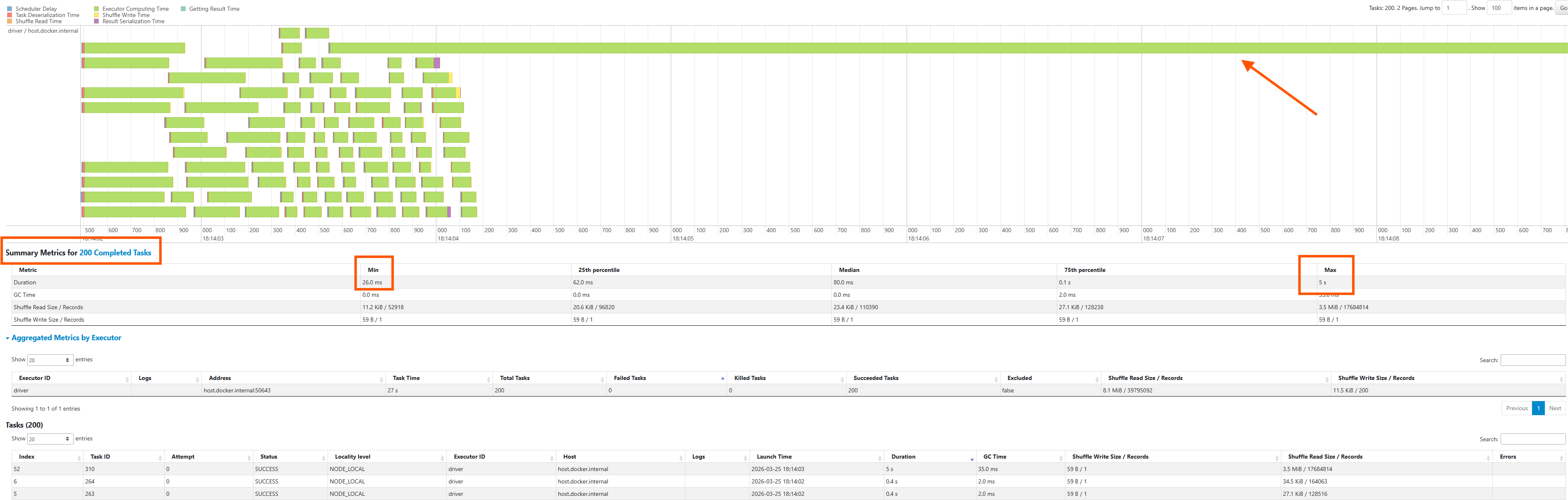
The task sorted by duration descending says it all:
- Task 191: 5s duration, 55ms GC time, 5.5 MiB / 17,684,914 records
- All other tasks: ~0.2s, ~4ms GC time, ~21 KiB / ~2,000 records
One task handles 17.6M records while 199 others handle ~2,000 each. The task timeline shows the two long red bars at the top — those are the skewed tasks holding everyone back.
Spark UI — With AQE
5 tasks, duration range: 3s → 7s (2× gap)
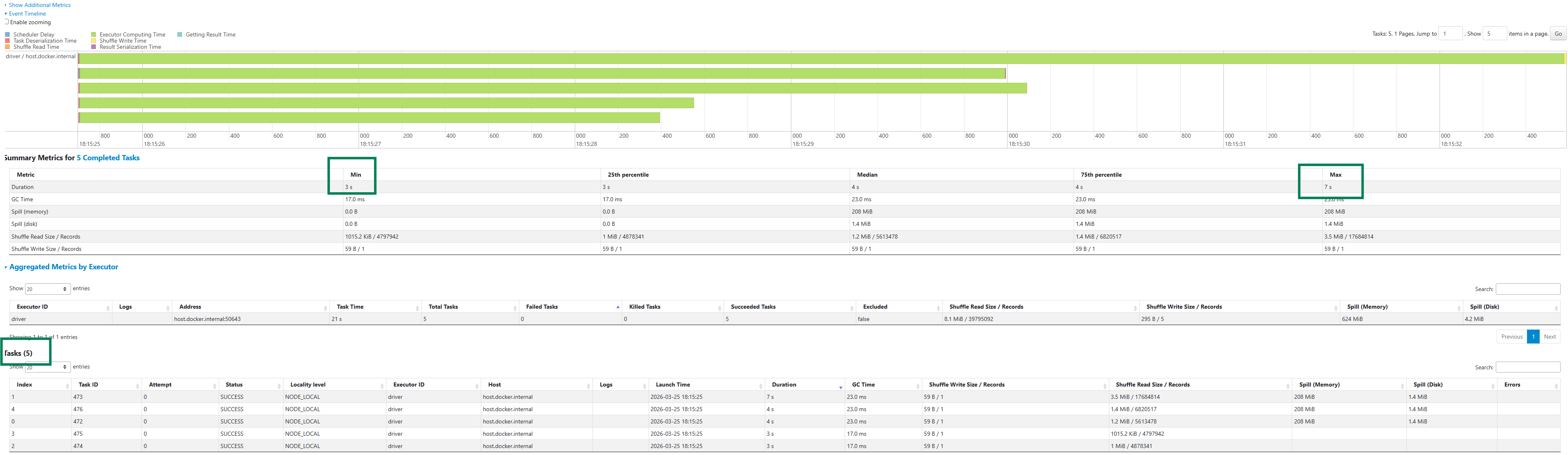
AQE detected the skewed partitions and redistributed the load:
- 5 tasks instead of 200 — AQE coalesced the small partitions and split the skewed one
- Min: 3s, Max: 7s — the extreme outlier is gone
- Task timeline shows similar bar lengths — uniform distribution
- The min/max gap collapsed from 190× to 2×
AQE didn’t fully eliminate the skew — one task still processes more data than others — but the 190× outlier became a 2× imbalance. That’s the realistic expectation on a single-executor local setup. On a multi-node cluster, the split sub-tasks run on separate executors in parallel, reducing wall time proportionally.
How the Split Works
AQE detects skewed partitions using two thresholds, both of which must be met:
A partition is skewed if:
  size > skewedPartitionFactor × median_partition_size
  AND
  size > skewedPartitionThresholdInBytes
For each skewed partition on the build side of a Hash Join, AQE splits it into sub-partitions and reads the corresponding range from the probe side:
Before: Partition 0 (8M rows) → 1 task → 1 executor → bottleneck

After (split into 4):
  Partition 0a (2M rows) → Executor A  ┐
  Partition 0b (2M rows) → Executor B  ├ parallel
  Partition 0c (2M rows) → Executor C  ┘
  Partition 0d (2M rows) → Executor D
Configuration
spark.conf.set("spark.sql.adaptive.skewJoin.enabled", "true")

// Partition is skewed if it's more than N× the median size (default: 5)
spark.conf.set("spark.sql.adaptive.skewJoin.skewedPartitionFactor", "5")

// AND if its absolute size exceeds this threshold (default: 256 MB)
spark.conf.set("spark.sql.adaptive.skewJoin.skewedPartitionThresholdInBytes", "268435456")
Critical Limitation: Hash Joins Only
AQE skew handling only works on Hash Joins (BHJ or Shuffle Hash Join). It cannot handle skew in Sort-Merge Joins — this is a fundamental mechanical constraint, not a gap in the implementation.
In a Hash Join, each partition is processed independently. AQE can split it and send sub-partitions to different executors. In a Sort-Merge Join, both sides must be co-located on the same executor — splitting one side without synchronizing the other breaks the join semantics.
When you have skew on a Sort-Merge Join, use manual salting:
val saltFactor = 50

val saltedLarge = largeDf
  .withColumn("salt", (rand() * saltFactor).cast(IntegerType))
  .repartition(col("salt"), col("join_key"))

val saltedSmall = smallDf
  .withColumn("salt", explode(array((0 until saltFactor).map(lit(_)): _*)))

saltedLarge.join(saltedSmall, Seq("join_key", "salt"))
// join_key=0 → (0,0), (0,1), ..., (0,49) → 50 executors in parallel
| Scenario | AQE handles it? | Alternative |
|---|---|---|
| Skew on Hash Join | ✅ Automatic | — |
| Skew on Sort-Merge Join | ❌ No | Manual salting |
Skew factor < skewedPartitionFactor |
❌ Below threshold | Lower the factor |
| Skew on RDD operations | ❌ Outside Catalyst | Repartition manually |
What AQE Manages vs. What You Still Own
| Optimization | AQE? | If Not, Who? |
|---|---|---|
| Coalesce small partitions post-shuffle | ✅ Automatic | — |
| SMJ → BHJ switch at runtime | ✅ Automatic | — |
| Split skewed partitions (Hash Joins) | ✅ Automatic | — |
| Small files before write | ❌ | coalesce() before write |
| Skew on Sort-Merge Joins | ❌ | Manual salting |
persist() / unpersist() strategy |
❌ | Developer responsibility |
Strategic repartition() |
❌ | Business/architecture decision |
RDD API (groupByKey, flatMap) |
❌ | Outside Catalyst entirely |
Production Configuration Reference
SparkSession.builder()
  // --- AQE Core ---
  .config("spark.sql.adaptive.enabled", "true")
  .config("spark.sql.shuffle.partitions", "600")

  // --- Feature 1: Coalescing ---
  .config("spark.sql.adaptive.advisoryPartitionSizeInBytes", "134217728")       // 128 MB
  .config("spark.sql.adaptive.coalescePartitions.minPartitionSize", "1048576")  // 1 MB floor

  // --- Feature 2: Join Switching ---
  .config("spark.sql.autoBroadcastJoinThreshold", "52428800")                   // 50 MB

  // --- Feature 3: Skew Join ---
  .config("spark.sql.adaptive.skewJoin.enabled", "true")
  .config("spark.sql.adaptive.skewJoin.skewedPartitionFactor", "5")
  .config("spark.sql.adaptive.skewJoin.skewedPartitionThresholdInBytes", "268435456")

  // --- Memory ---
  .config("spark.executor.memoryOverhead", "4g")
  .config("spark.executor.extraJavaOptions", "-XX:+UseG1GC -XX:G1HeapRegionSize=16m")
  .getOrCreate()
Spark UI Verification Checklist
| Feature | Where to look | What confirms it’s working |
|---|---|---|
| Coalescing | SQL tab → Physical Plan | AQEShuffleRead node: number of partitions « shuffle.partitions |
| Join switching | SQL tab → Physical Plan | BroadcastHashJoin + BroadcastExchange where SMJ was planned |
| Skew handling | Stages tab → task list sorted by duration | Min/max duration gap collapses; no single outlier dominating |
Key Takeaways
- AQE re-optimizes at every shuffle boundary using real measured statistics — not estimates
- Feature 1 (Coalescing): Set
shuffle.partitionshigh, let AQE reduce it to the actual required count. Proof:AQEShuffleReadin the physical plan. - Feature 2 (Join Switching): AQE catches cases where Catalyst over-estimated table size and silently switches SMJ → BHJ. Proof:
BroadcastHashJoinwhere SMJ was planned, plus AQE can apply multiple features simultaneously at the same boundary. - Feature 3 (Skew Join): Automatic for Hash Joins — the min/max task duration gap is your metric. Sort-Merge Join skew still requires manual salting.
- AQE only covers the DataFrame/Dataset API — RDD operations are outside Catalyst’s reach
- All three features activate with a single config line:
spark.sql.adaptive.enabled = true
Which of these three features has had the most impact in your pipelines? For most teams it’s Coalescing — but the answer changes dramatically depending on your join patterns and data distributions. Drop your numbers in the comments.